Using an API (an application programming interface) is a very popular tool for data scientists to pull data from a public source. I’ve done a bit of web scraping in previous blogposts where I collected data from for example Wikipedia and the Olympian Database. However, I’d much prefer using APIs whenever possible, this way the creator has more control of what data they want to share and how it is packaged. The most common APIs use a RESTful approach where the interface and communication between you and the server the data is stored on follows a predictable approach and maintains some common standards. Most RESTful APIs return data in JSON format. In this blogpost I want to show you a simple way to interact with a RESTful API through Python and of course we’ll do some analyses on the data we collect.

The API we will be working with here is the New York Times Books API. This API provides us with access to the current and previous (up to 2008) New York Times Best Sellers lists. It allows ut to download each individual list (both fiction, non-fiction, children’s, etc), including ones that are no longer updated (such as the monthly lists on Espionage and Love & Relationships). Let’s keep it simple for now and only focus on the main list on fiction, called the Combined Print & E-Book Fiction list which appears as the list on the home page of the Best Sellers webpage.

Let’s first setup our Python environment. We’ll use pandas to store the results for easy data wrangling and the numpy module to get access to the np.nan functionality to denote missing values. The requests module deals with the the API calls to the server. We’ll get into that. Since the NYT APIs require a personal API key (a key I don’t want to share on the internet), I’ll store my API key in a “secrets” file, in this case a .secrets.yml YAML file that easily stores these kinds of data. If you’re not familiar with YAML, it’s the same format that Hugo, RMarkdown, and Quarto documents use to define settings and parameters. To parse YAML files, we can use the yaml module. We’ll also be dealing with a few date formats, so I’ll import a few items from the datetime module. Finally, we’ll load the time module. Many APIs are “rate limited” to avoid users from submitting too many requests in a short amount of time and clogging up the server. The time module has a sleep() function that lets us wait a given number of seconds before proceding. This way we can avoid exceeding the API rate limit and interrupting the data collection.

import pandas as pd
import numpy as np
import requests
import yaml
from datetime import datetime, timedelta
import time

So in proper Python fashion, we’ll encapsulate the functions as much as possible. The NYT Books API lets us download historical versions of the Best Seller lists. Therefore, we need first to get a list of dates that we can use for our API request. For this we’ll make a simple function that takes the start and end date of the timeframe of interest which we can set by default to provide a list going back 52 weeks from today. As well as the frequency (so that we can more easily and quickly download monthly lists if we wanted to). The exact date Best Seller list was released is not important since the API will return the latest list at the requested date. To generate the date list we’ll use a simple pd.date_range() function, and we’ll format them in a default string format using a list comprehension and the strftime() function from the datetime module.

def get_list_of_dates(
    start=datetime.today() - timedelta(weeks=52), 
    end=datetime.today(), 
    frequency="W"
  ):
  """
  Generate a list of dates
  """
  
  date_list = pd.date_range(start, end, freq=frequency)
  date_list_str = [x.strftime("%Y-%m-%d") for x in date_list]
  return date_list_str

Now that we have a function that will provide a list of dates, the next ingredient we need is the API key. The NYT Books API requires a personal API key to authenticate your request. Since this key is personal I won’t upload it the internet, but instead I stored it in a .secrets.yml file that I put in my .gitignore file to avoid storing it in Git log. We’ll use the functionality from the yaml module to parse the file. The function will return the API key as a string.

def _get_api_key(path="./.secrets.yml"):
  """
  Get the API key from the secrets file
  """
  with open(path, "r") as stream:
    secrets = yaml.safe_load(stream)
  nyt_api_key = secrets["API"]["NYT"]
  return nyt_api_key

Now we’re ready to generate a single API query. To obtain the list we’re interested in, we can follow the template laid out on the NYT Books API documentation. The request starts with a base url (in this case https://api.nytimes.com/svc/books/v3). Then we’ll specify both the date and list type, both of which are defined in the input arguments to the generate_request() function. By default we request the “fiction” list (that defaults to the combined-print-and-e-book-fiction list), providing “non-fiction” as input to this argument would default to the combined-print-and-e-book-nonfiction list. Any other list needs to use the specific name (we’ll get back to that later). Finally, we use the _get_api_key() function we defined earlier to get the last parameter we need to the finalize the query.

def generate_request(list="fiction", date="current"):
  """
  Generate the API request url
  """
  
  base = "https://api.nytimes.com/svc/books/v3"
  
  if list == "fiction":
      list_spec = f"/lists/{date}/combined-print-and-e-book-fiction.json"
  elif list == "non-fiction":
      list_spec = f"/lists/{date}/combined-print-and-e-book-nonfiction.json"
  else:
      list_spec = f"/lists/{date}/{list}.json"
      
  nyt_api_key = _get_api_key()
  
  api_url = f"{base}{list_spec}?api-key={nyt_api_key}"
  
  return api_url

Now we get to the part where we actually download some data using the functions we created earlier. We can again define the list we’re interested in and the date in the input arguments to this function. These will trickle down to the lower level functions. We first generate the URL by using the generate_request() function. Then we’ll use the requests module to obtain the response from the server and get the returned data in a JSON format. The JSON contains a bunch of information, but we’re mostly interested in the books part that actually lists the books in order of appearance on the specified list on the specified date. One of the other information that is not in the books field is the published_date field that shows when the list was last updated. We can parse this date so we can include it in the data frame that will be returned in the end. The books field contains some information is not particularly interesting (like the size of the book cover and the buy links shown on the NYT website).

We’ll parse some the data, i.e. make the "title" field title-case, replace zeroes that denote that a book wasn’t in the list with np.nan, calculate the difference in ranking between each week, and add the date the list was published. Finally we’ll reorder the columns and return a data frame.

def api_request(list="fiction", date="current"):
  """
  Extract the data from the API
  """
  
  url = generate_request(list=list, date=date)
  
  response = requests.get(url)
  json_raw = response.json()
  
  nyt_list_json = json_raw["results"]["books"]
  list_publish_date = json_raw["results"]["published_date"]
  
  df_all = pd.DataFrame().from_dict(nyt_list_json)
  
  cols_to_drop = [
      "book_image",
      "book_image_width",
      "book_image_height",
      "isbns",
      "buy_links",
  ]
  
  df = df_all.drop(columns=cols_to_drop).copy()
  df["title"] = df["title"].str.title()
  df["rank_last_week"].replace({0: np.nan}, inplace=True)
  df["list_publication_date"] = list_publish_date
  
  df_out = df[["rank", "rank_last_week", "title", "author", 
    "weeks_on_list", "list_publication_date"]].copy()
  
  return df_out

Now, each of the functions above dealt with performing a single API request. Since we are interested in obtaining an historical dataset, we should run the API request for each of the weeks we returned in the get_list_of_dates() function. In the download_bestseller_lists() function, we’ll first get the list of dates. Then we’ll loop through the list of dates going back roughly 5 years. In each iteration we’ll run the api_request() function for the specified date and concatenate the result with the existing data frame. Then, in order to avoid hitting the API rate limit we’ll wait for 12 seconds, the NYT Books API is rate limited at 500 requests per day and 5 requests per minute so we need to wait 12 seconds between each request to avoid hitting the rate limit. Finally, we’ll run this download_bestseller_lists() function for the Fiction list, and save the output in a CSV file.

def download_bestseller_lists(
      list_type="fiction", 
      start_date=datetime.today() - timedelta(weeks=5*52), 
      end_date=datetime.today(),
      save=True,
      return_df=False
  ):
  """
  Download the Best Seller list from a given date
  """
  date_list = get_list_of_dates(start=start_date, end=end_date)
  
  n_dates = len(date_list)
  print(f"Number of requests: {n_dates}")
  print(f"Estimated download time: {n_dates * 12}s or {n_dates * 12 / 60}min")
  
  df_nyt_list = pd.DataFrame()
  for i in date_list:
      print(f"Extracting {list_type} list at date {i}")
      df_nyt_list = pd.concat([df_nyt_list, api_request(list=list_type, date=i)])
      time.sleep(12)
      
  if save:
    df_nyt_list.to_csv(f"./data/nyt_list_{list_type}.csv", index=False)
  
  if return_df:
    return df_nyt_list

download_bestseller_lists(list_type="fiction")

Now that we’ve done the hard work in Python, let’s do some data visualization in R using ggplot and a few other {tidyverse} and plotting related packages ({ggtext} and {patchwork}). Since the download_bestseller_lists() function in Python also saved the file, we can easily load it into R. Since I’m using the {reticulate} package to create this, I could have also used the py$<variable name> functionality, but since the API call takes a lot of time to run, this seemed easier.

data <- read_csv("./data/nyt_list_fiction.csv") |>
  glimpse()

Rows: 3900 Columns: 6
── Column specification ────────────────────────────────────────────────────────
Delimiter: ","
chr  (2): title, author
dbl  (3): rank, rank_last_week, weeks_on_list
date (1): list_publication_date

ℹ Use `spec()` to retrieve the full column specification for this data.
ℹ Specify the column types or set `show_col_types = FALSE` to quiet this message.

Rows: 3,900
Columns: 6
$ rank                  <dbl> 1, 2, 3, 4, 5, 6, 7, 8, 9, 10, 11, 12, 13, 14, 1…
$ rank_last_week        <dbl> NA, NA, NA, 5, 1, 4, 8, NA, 10, NA, 3, NA, 9, NA…
$ title                 <chr> "Vince Flynn: Red War", "An Absolutely Remarkabl…
$ author                <chr> "Kyle Mills", "Hank Green", "Kate Atkinson", "Ke…
$ weeks_on_list         <dbl> 1, 1, 1, 16, 2, 3, 3, 1, 4, 1, 31, 15, 8, 1, 7, …
$ list_publication_date <date> 2018-10-14, 2018-10-14, 2018-10-14, 2018-10-14,…

As mentioned, the dataset we downloaded does not include all history of the Best Sellers list due to the API rate limit. Instead we specified that we want to look about 5 years back, let’s see what the earliest to latest dates in the dataset are.

data |>
  summarise(
    from = min(list_publication_date),
    to = max(list_publication_date)
  )

# A tibble: 1 × 2
  from       to        
  <date>     <date>    
1 2018-10-14 2023-10-01

The purpose of this post is mostly to show the implementation of an API call in Python, but I want to make some plots anyway because it’s fun. Let’s first look at what book has spend the longest on the Best Sellers list. Just to make it easier to determine the book, we’ll create a composite variable of both the book author and title before plotting and take the 20 books that have the most occurences on the list using the count() function and then use the slice_max() to limit the dataset to 20.

data |>
  count(author, title, name = "n_weeks_on_list") |>
  mutate(book_label = str_glue("{author} - {title}")) |>
  slice_max(order_by = n_weeks_on_list, n = 20) |>
  ggplot(aes(x = n_weeks_on_list, y = reorder(book_label, n_weeks_on_list))) +
  geom_col(fill = "#5D7B92") +
  geom_text(aes(label = n_weeks_on_list),
    nudge_x = -7,
    color = "white", fontface = "bold"
  ) +
  geom_vline(xintercept = 0, linewidth = 1) +
  labs(
    title = "Which books have spent the longest<br>on the NYT Best Sellers list?",
    x = NULL,
    y = NULL
  ) +
  scale_x_continuous(
    position = "top",
    labels = ~ str_glue("{.x} wk"),
    expand = expansion(add = c(0, 20))
  ) +
  theme_minimal() +
  theme(
    plot.title.position = "plot",
    plot.title = element_markdown(size = 18, face = "bold"),
    panel.grid.major.y = element_blank()
  )

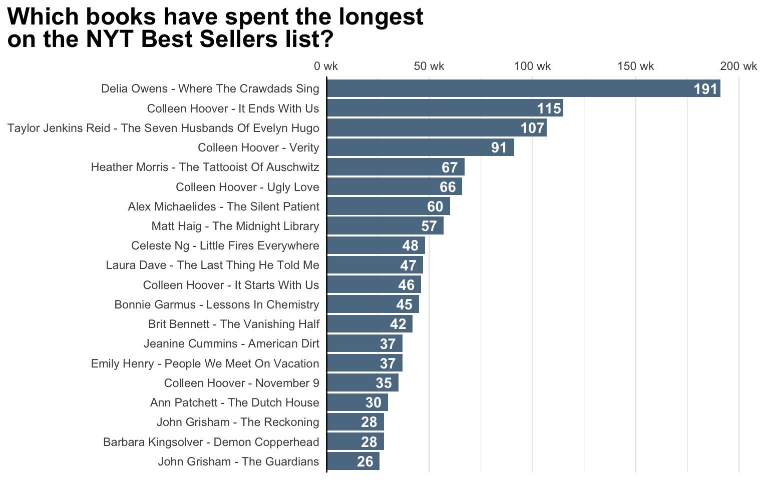
It looks like Where The Crawdads Sing by Delia Owens has appeared a total of 193 times on the list in the past 5 years. The number two (It Ends With Us) follows with 115 weeks, but after inspection of the data that book is currently in the list, so may yet make up some ground.

Let’s also look at which authors have had the largest number of books in the list in the past 5 years using roughly the same approach.

data |>
  distinct(author, title) |>
  count(author, name = "n_books_in_list") |>
  slice_max(order_by = n_books_in_list, n = 10) |>
  ggplot(aes(x = n_books_in_list, y = reorder(author, n_books_in_list))) +
  geom_col(fill = "#5D7B92") +
  geom_text(aes(label = n_books_in_list),
    nudge_x = -1,
    color = "white", fontface = "bold"
  ) +
  geom_vline(xintercept = 0, linewidth = 1) +
  labs(
    title = "Which authors have the most books<br>on the NYT Best Sellers list?",
    x = NULL,
    y = NULL
  ) +
  scale_x_continuous(
    position = "top",
    labels = ~ str_glue("{.x} books"),
    expand = expansion(add = c(0, 5))
  ) +
  theme_minimal() +
  theme(
    plot.title.position = "plot",
    plot.title = element_markdown(size = 18, face = "bold"),
    panel.grid.major.y = element_blank()
  )

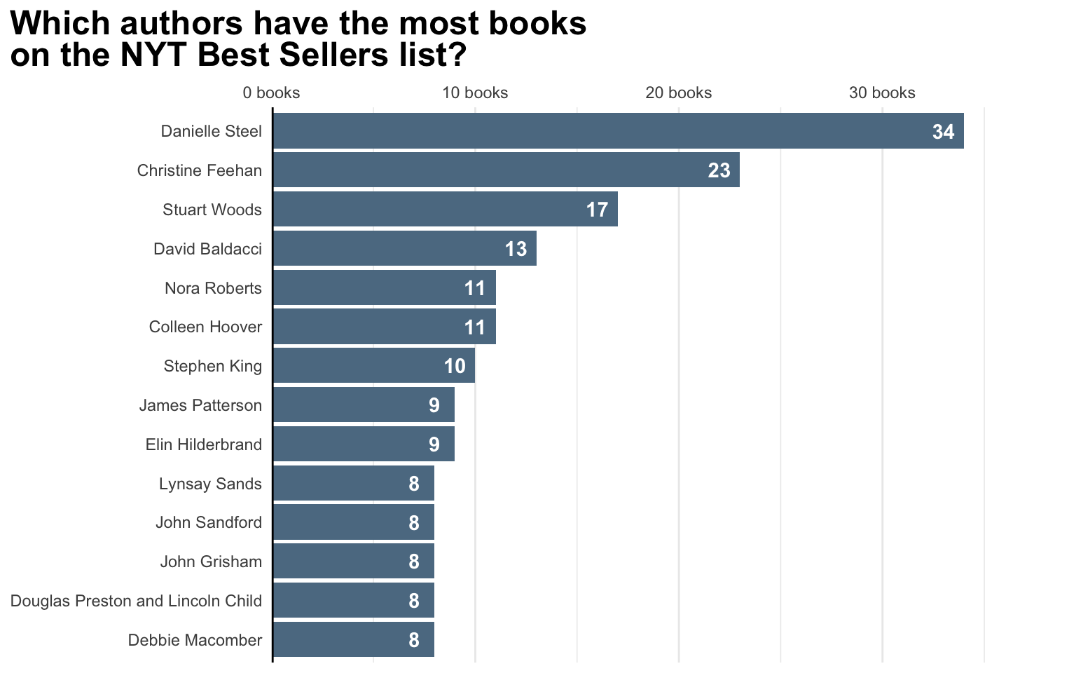
This genuinely surprised me, I had expected some authors to have maybe 6 or 7 books on the list, but it turns out there are some really prolific authors out there, with Danielle Steel definitely taking the top spot. According to her separate (!) bibliography page on Wikipedia she publishes several books a year to make a total of 190 published books, including 141 novels. Wikipedia also mentions a “resounding lack of critical acclaim”, which just emphasizes the point that the New York Times Best Sellers list is not necessarily a mark of quality, but rather of popularity, although one would hope good books are also the books that sell well. Note that some authors have received critical acclaim and have published multiple popular books such as Colleen Hoover and Stephen King in the plot above.

Since we have essentially time series data, we could also plot the trajectory of a book. So let’s take the book that spent the longest on the Best Sellers list in our timeframe: Where The Crawdads Sing. We can plot rank on the list over time. We’ll use the geom_bump() function from the {ggbump} package to get a nicer-looking curve. Since geom_path() and geom_bump() will show a continuous line for missing values and dropping those empty values looks ugly, we’ll hide the weeks where the book wasn’t on the Best Sellers list in an area below the plot.

title_of_interest <- "Where The Crawdads Sing"

data |>
  filter(title == title_of_interest) |>
  right_join(data |> select(list_publication_date) |> distinct(),
    by = "list_publication_date"
  ) |>
  replace_na(list(rank = 16)) |>
  ggplot(aes(x = list_publication_date, y = rank)) +
  geom_hline(yintercept = 1, color = "grey", linetype = "dotted") +
  ggbump::geom_bump(linewidth = 1, color = "#5D7B92") +
  geom_rect(aes(
    xmin = min(data$list_publication_date),
    xmax = max(data$list_publication_date),
    ymin = 15.2, ymax = Inf
  ), fill = "grey40") +
  geom_text(data = tibble(), aes(
    x = mean(data$list_publication_date), y = 15.75,
    label = "Not on list"
  ), color = "white") +
  labs(
    title = str_glue("How _{title_of_interest}_ ranked over time"),
    x = NULL,
    y = "Position on Best Sellers list"
  ) +
  scale_y_continuous(
    trans = "reverse",
    breaks = seq(15),
    expand = expansion(add = c(0.5, 0))
  ) +
  coord_cartesian(clip = "off") +
  theme_minimal() +
  theme(
    plot.title.position = "plot",
    plot.title = element_markdown(
      size = 18, face = "bold",
      padding = margin(b = 10)
    ),
    panel.grid.minor.y = element_blank()
  )

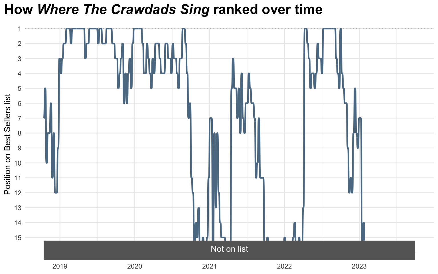
That is quite an impressive trajectory. There are a few moments where the book leaves the Best Sellers list, but it had a spot on the list every year from 2018 when the book was published to 2023.

The jump in the plot above that happens in 2022 seemed very remarkable, jumping from spot 13 to 1 within a week. I was wondering if that had anything to do with the release of the movie adaptation. So let’s have a look. The movie was released on July 15th, 2022. Let’s also look at a few other books I know were on the Best Sellers list that have gotten an adaptation. This is just anecdotal and hand-picked evidence of course so needs to be taken with a grain of salt. Perhaps another time I’ll find a more systematic way of testing this. In addition to Where The Crawdads Sing, I’ve picked two other movies and three TV series. The other two movies are Bird Box released in late 2018 and It Chapter Two, the second installment of the adaptation of It by Stephen King. For the TV series I’ll look at the wonderful Normal People based on the novel by Sally Rooney, initially released in 2020, The Outsider also based on a book by Stephen King, and The Handmaid’s Tale based on the book by Margaret Atwood. In the plots below the vertical dashed line indicates the release date of the adaptation.

titles_w_adaptation <- tribble(
  ~title, ~screen_release_date,
  "Where The Crawdads Sing", "2022-07-15",
  "Bird Box", "2018-12-14",
  "It", "2019-09-06",
  "Normal People", "2020-04-26",
  "The Outsider", "2020-01-06",
  "The Handmaid'S Tale", "2019-6-5"
)

rplot <- list()
for (i in seq_len(nrow(titles_w_adaptation))) {
  book_title <- titles_w_adaptation |>
    slice(i) |>
    mutate(title = str_replace(title, "'S", "'s")) |>
    pull(title)

  rplot[[i]] <- data |>
    right_join(titles_w_adaptation |>
                 slice(i), by = "title") |>
    right_join(data |> select(list_publication_date) |> distinct(),
      by = "list_publication_date"
    ) |>
    replace_na(list(rank = 16)) |>
    ggplot(aes(x = list_publication_date, y = rank)) +
    geom_hline(yintercept = 1, color = "grey", linetype = "dotted") +
    ggbump::geom_bump(linewidth = 1, alpha = 0.25) +
    geom_rect(aes(
      xmin = min(data$list_publication_date),
      xmax = max(data$list_publication_date),
      ymin = 15.2, ymax = Inf
    ), fill = "grey40", show.legend = FALSE) +
    geom_text(data = tibble(), aes(
      x = mean(data$list_publication_date), y = 15.75,
      label = "Not on list"
    ), color = "white") +
    geom_vline(aes(xintercept = as.Date(screen_release_date)),
      linewidth = 1, linetype = "dashed"
    ) +
    labs(
      title = str_glue("Ranking of _{book_title}_"),
      x = NULL,
      y = "Rank on list",
      color = NULL
    ) +
    scale_y_continuous(
      trans = "reverse",
      breaks = seq(15),
      expand = expansion(add = c(0.5, 0))
    ) +
    coord_cartesian(clip = "off") +
    theme_minimal() +
    theme(
      plot.title.position = "plot",
      plot.title = element_markdown(
        size = 14, face = "bold",
        padding = margin(b = 10)
      ),
      panel.grid.minor.y = element_blank(),
      legend.position = "bottom",
      legend.direction = "vertical"
    )
}

(rplot[[1]] + rplot[[2]]) /
  (rplot[[3]] + rplot[[4]]) /
  (rplot[[5]] + rplot[[6]]) +
  plot_annotation(
    caption = "Vertical dashed line indicates the adaptation's release date"
  ) &
  theme(plot.caption = element_markdown(size = 12))

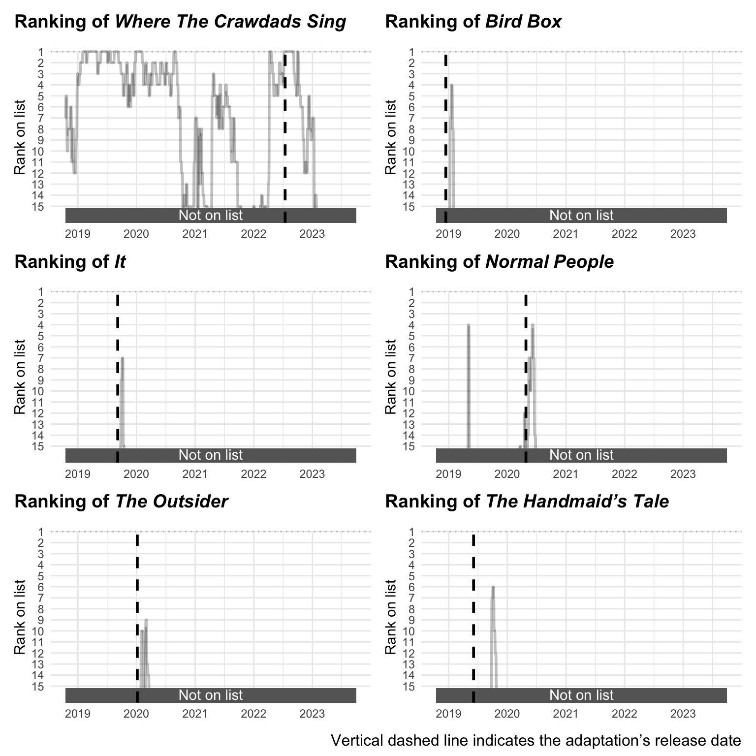
It seems that for Where The Crawdads Sing, the movie release ensured that the book remained at number 1 on the Best Sellers list for a while, even though the book was already doing very well in the list before the movie release. For both Bird Box and It their movie releases seemed to have caused a boost in sales of the book that made them reappear in the list for a short time. I’d guess the fact that the book Where The Crawdads Sing was already very popular prior to the movie release caused a boost in popularity that lingered longer. Both Bird Box and It had a brief reappearance in the list following their movie release, but I’d guess that a publisher cannot rely on a successful movie release (like Bird Box or It) to boost the sales of a book. It cannot compensate for the success of an already popular and well-received book like Where The Crawdads Sing.

For the TV series I looked at, the pattern looks very similar to the previous two movies. The book Normal People had already appeared briefly on the Best Sellers list, but reappeared after the initial release of the popular HBO series for slightly longer. The same is true for both The Outsider and The Handmaid’s Tale. Although The Handmaid’s Tale was initially published in 1985, it reappeared briefly in the list following the release of the third season of the HBO series. The Outsider was initially published in 2018, and it’s series adaptation release in early 2020 cause a short boost in popularity also.

This was a fun little post, I hope this little tutorial on the practical implementation of an API call was useful. If you want to explore other lists other than the “Combined Print and E-Book Fiction” list, the code below shows how you can download all lists available in the API using a similar approach as above.

def get_nyt_lists(save=True, return_df=False):
  """
  Get an overview of all best-seller lists
  """

  response = requests.get(
    f"https://api.nytimes.com/svc/books/v3/lists/names.json?api-key={_get_api_key()}"
  )
  json_raw = response.json()
  list_names = json_raw["results"]
  df_names = pd.DataFrame().from_dict(list_names)

  if save:
    df_names.to_csv(f"./data/nyt_all_lists.csv", index=False)
    
  if return_df:
    return df_names

get_nyt_lists()

If you wish to explore other APIs, there’s a ton of public APIs that you can explore using the approach discussed here. Thanks for reading, and thanks sticking all the way through! Happy coding!