Today I want to share a project that deals with data scientist’s favorite kind of data: date- and timedata involving time zones and daylight savings time. Who doesn’t love it?

This project stems from a discussion I had with my family about living up north in Norway and when the days become longer than in the Netherlands. Intuitively, one might think that because of the prevailing snow and cold in March and occasionally April this corresponds with shorter day length. We can look at the data and see what the length of day and sunset time trajectories actually look like. Perhaps we can learn something about working with date- and timedata.

As always, let’s use R to make the plots, but I think Python is a bit better suited to do the data wrangling in this case. First, we’ll load the packages we’ll need here. We’ll use the default packages like {tidyverse} and {ggtext}, but in addition (since we’ll be dealing with time data) we’ll also load the {lubridate} package. I’m writing this in Quarto so the {reticulate} package does not need to be loaded directly to use the Python code blocks, but we’ll use it using the :: syntax later to easily get the results back to R using the py$<variable name> functionality.

library(tidyverse)
library(lubridate)
library(ggtext)

reticulate::use_virtualenv("./.venv", required = TRUE)

theme_custom <- function(...) {
  ggthemes::theme_fivethirtyeight(...) +
    theme(
      plot.background = element_rect(fill = "transparent"),
      panel.background = element_rect(fill = "transparent"),
      legend.background = element_rect(fill = "transparent"),
      legend.key = element_rect(fill = "transparent")
    )
}

For the Python part, we’ll use pandas as usual, the datetime and time module to deal with date- and timedata. The dateutil module to deal with time zones. And to get the actual raw data we’ll use the astral module to get the sunrise and sunset times for different locations. Unfortunately, not all cities are included, it includes all capital cities plus some additional cities in the UK and USA. To get the coordinates for the cities we want to look at, we’ll use the geopy module which allows you to look up the longitude, latitude of a given location without needing to create an account somewhere or dealing with an API (directly). To deal with some wrangling of strings we’ll use the re module.

import pandas as pd
from datetime import date, timedelta, datetime
import time
from dateutil import tz
from astral import LocationInfo
from astral.sun import sun
from geopy.geocoders import Nominatim
import re

For this project we’ll collect a number of variables related to sunrise and sunset for different locations throughout the year. The astral module makes this very easy, and in order to keep things clean and efficient we’ll create a function to efficient collect this data. We’ll write it in such a way that it can collect a number of locations within one function call using a list input (which isn’t the cleanest, but works quite well here). We’ll provide the list of cities we want to analyze in the form '<region>/<city>' to avoid any possible misconceptions (e.g. Cambridge, Cambridgeshire in the UK or Cambridge, MA in the US). We’ll then extract the coordinates for that location using the geopy module. We’ll also supply the reference time zone (for this project Central Europe). The astral module has a known issue when dusk happens past midnight. So we’ll extract everything in UTC and convert it to the time zone of interest later. We’ll collect the data throughout the year for the various locations in a loop. And we’ll cycle through the year using a while loop. We’ll also collect the difference in time from the Daylights Savings Time. We’ll convert it to the time zone of interest using the _convert_timezone() function. In the final data frame we’ll only get the times (not the dates) so in case the dusk happens past midnight, we’ll consider that “no dusk takes place this day” instead of having it happen “early in the morning the same day”, implemented in the _fix_dusks_past_midnight() function. This will help with the plots later. Finally we’ll convert some of the variables to a format that’ll make it easy to deal with in R later.

def _convert_timezone(x, to_tz=tz.tzlocal()):
    """
    Convert the default time zone to local
    """

    x_out = x.apply(lambda k: k.astimezone(to_tz))

    return x_out


def _fix_dusks_past_midnight(sunset, dusk):
    """
    Replace the dusk time with NaN if it's past midnight
    """

    sunset_dt = datetime.strptime(sunset, "%H:%M:%S")
    dusk_dt = datetime.strptime(dusk, "%H:%M:%S")

    if dusk_dt < sunset_dt:
        dusk_out = "23:59:59"
    else:
        dusk_out = dusk_dt.strftime("%H:%M:%S")

    return dusk_out


def get_sun_data(
    cities=["Norway/Oslo", "Netherlands/Amsterdam"],
    ref_tz="Europe/Berlin"
):
    """
    Get sunset data from location
    """

    geolocator = Nominatim(user_agent="sunset-sunrise-app")

    df = pd.DataFrame()
    for i, city in enumerate(cities):
        df_tmp = pd.DataFrame()

        loc = geolocator.geocode(city)
        city_loc = LocationInfo(
            timezone=city, latitude=loc.latitude, longitude=loc.longitude
        )

        start_date = datetime.strptime(date.today().strftime("%Y-01-01"), "%Y-%m-%d")
        end_date = datetime.strptime(date.today().strftime("%Y-12-31"), "%Y-%m-%d")
        delta = timedelta(days=1)
        while start_date <= end_date:
            s = sun(city_loc.observer, date=start_date)
            s["dst"] = time.localtime(start_date.timestamp()).tm_isdst
            df_tmp = pd.concat([df_tmp, pd.DataFrame(s, index=[0])])
            start_date += delta
        df_tmp["city_no"] = i + 1
        df_tmp["location"] = city_loc.timezone
        df_tmp["lat"] = loc.latitude
        df_tmp["long"] = loc.longitude
        df = pd.concat([df, df_tmp])

    df.reset_index(drop=True, inplace=True)
    df["date"] = df["noon"].dt.strftime("%Y-%m-%d")
    df["dst"] = df["dst"].shift(-1, fill_value=0)
    df["city"] = df["location"].apply(lambda x: re.findall("\\/(.*)", x)[0])

    cols = ["dawn", "sunrise", "noon", "sunset", "dusk"]
    df[cols] = df[cols].apply(lambda k: _convert_timezone(k, to_tz=ref_tz))
    df[cols] = df[cols].apply(lambda k: k.dt.strftime("%H:%M:%S"))
    df["dusk"] = df.apply(
        lambda k: _fix_dusks_past_midnight(sunset=k["sunset"],
            dusk=k["dusk"]), axis=1
    )

    return df

Let’s run this function once for Oslo, Amsterdam, Warsaw, and Madrid and once for only Oslo and Amsterdam. Amsterdam and Warsaw are roughly on the same latitude, Madrid and Oslo are on opposite ends. Both Warsaw and Madrid are also on either end of the central European time zone. Let’s also look at the output.

df = get_sun_data(
  ["Norway/Oslo", "Netherlands/Amsterdam",
  "Poland/Warsaw", "Spain/Madrid"]
  )
df_deux = get_sun_data(["Norway/Oslo", "Netherlands/Amsterdam"])

print(df.info(), df.head())

<class 'pandas.core.frame.DataFrame'>
RangeIndex: 1460 entries, 0 to 1459
Data columns (total 12 columns):
 #   Column    Non-Null Count  Dtype  
---  ------    --------------  -----  
 0   dawn      1460 non-null   object 
 1   sunrise   1460 non-null   object 
 2   noon      1460 non-null   object 
 3   sunset    1460 non-null   object 
 4   dusk      1460 non-null   object 
 5   dst       1460 non-null   int64  
 6   city_no   1460 non-null   int64  
 7   location  1460 non-null   object 
 8   lat       1460 non-null   float64
 9   long      1460 non-null   float64
 10  date      1460 non-null   object 
 11  city      1460 non-null   object 
dtypes: float64(2), int64(2), object(8)
memory usage: 137.0+ KB
None        dawn   sunrise      noon    sunset  ...       lat      long        date  city
0  08:21:36  09:19:09  12:20:15  15:22:01  ...  59.91333  10.73897  2023-01-01  Oslo
1  08:21:19  09:18:39  12:20:43  15:23:29  ...  59.91333  10.73897  2023-01-02  Oslo
2  08:20:57  09:18:04  12:21:11  15:25:01  ...  59.91333  10.73897  2023-01-03  Oslo
3  08:20:31  09:17:24  12:21:38  15:26:37  ...  59.91333  10.73897  2023-01-04  Oslo
4  08:20:01  09:16:39  12:22:06  15:28:17  ...  59.91333  10.73897  2023-01-05  Oslo

[5 rows x 12 columns]

Here’s where we’ll define a function to get everything into R and create a data frame we can work with so we can reuse it. We’ll first reorder to columns to something sensible. We’ll convert the date and time columns to their respective variable types, and we’ll the length of day by subtracting the sunset time from the sunrise and get it into a time variable. Finally, we’ll sort the city variable by the order by which they were listed.

parse_sun_data <- function(df) {
  #' Get the data frame from Python into R

  data <- tibble(df) |>
    relocate(c("city", "date"), .before = "dawn") |>
    mutate(
      date = parse_date(date, "%Y-%m-%d"),
      across(dawn:dusk, ~ parse_time(.x, format = "%H:%M:%S")),
      day_length = hms::as_hms(sunset - sunrise),
      city = fct_reorder(city, city_no)
    )

  return(data)
}

Let’s have a look at when sunset happens throughout the year for these cities. I deliberately picked a few cities on extreme ends of the Central European time zone to show the variety within a single time zone. We’ll include the DST also.

data <- parse_sun_data(reticulate::py$df)

data |>
  ggplot(aes(x = date, y = sunset, color = city, group = city)) +
  geom_line(
    linewidth = 2, lineend = "round",
    key_glyph = "point"
  ) +
  labs(
    x = NULL,
    y = "Sunset time",
    color = NULL
  ) +
  scale_x_date(labels = scales::label_date(format = "%B")) +
  ggthemes::scale_color_tableau(
    guide = guide_legend(override.aes = list(size = 4))
  ) +
  theme_custom()

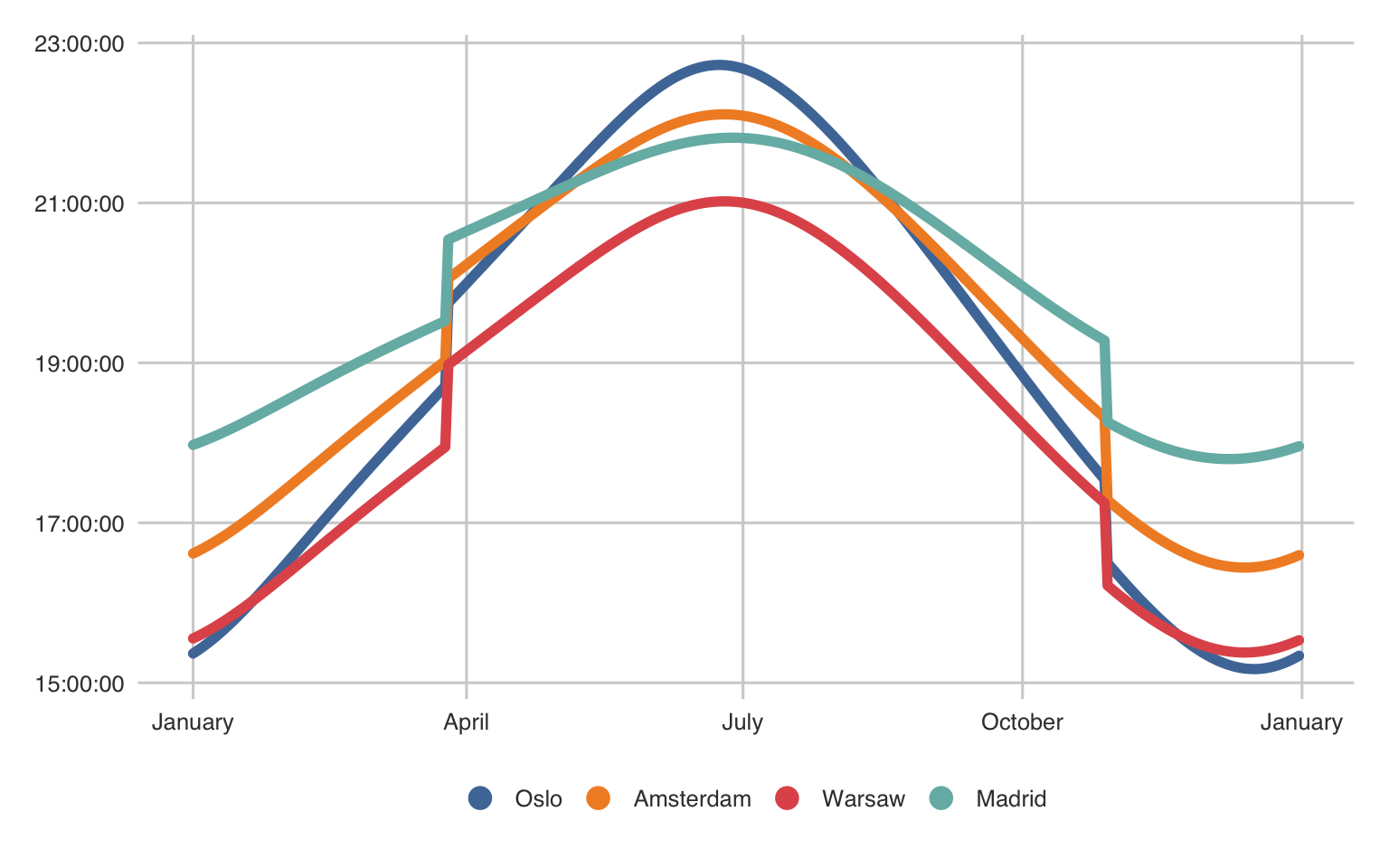
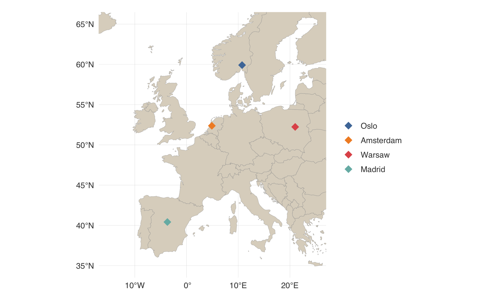
As expected, the latitude (how far north or south a location is) has the most to say about sunset times in summer in winter. Oslo has both the earliest and latest sunsets in winter and summer. And also predictable, the longitude (how far east or west a location is) merely shifts the curve up or down. Madrid has later sunsets in summer than Warsaw (which is further north) but also later sunsets in winter and a flatter curve overall. Oslo has a much steeper curve than e.g. Amsterdam while simultaneously also having the curve slightly shifted due to Oslo being further east than Amsterdam. The plot below shows the locations of of the cities in this analysis.

rnaturalearth::ne_countries(
  scale = "medium",
  returnclass = "sf",
  continent = "Europe"
) |>
  ggplot() +
  geom_sf(color = "grey60", fill = "#DDD5C7", linewidth = 0.1) +
  geom_point(
    data = data |> distinct(city, lat, long),
    aes(x = long, y = lat, color = city),
    shape = 18, size = 4
  ) +
  labs(color = NULL) +
  ggthemes::scale_color_tableau() +
  coord_sf(xlim = c(-15, 25), ylim = c(35, 65)) +
  theme_custom() +
  theme(
    legend.position = "right",
    legend.direction = "vertical",
    panel.grid.major = element_line(size = 0.1)
  )

Perhaps we can have a look at day length to get a better reflection of the isolated effect of latitude. To make the plot more legible, we’ll use only 2 cities this time.

We’ll create the plot using the geom_ribbon() function to shade the area between sunrise and sunset.

parse_sun_data(reticulate::py$df_deux) |>
  ggplot(aes(
    xmin = date, x = date, xmax = date,
    ymin = sunrise, y = noon, ymax = sunset,
    fill = city, color = city, group = city
  )) +
  geom_hline(
    yintercept = parse_time("12:00", "%H:%M"),
    linewidth = 1
  ) +
  geom_ribbon(alpha = 0.5, color = NA, key_glyph = "point") +
  labs(
    x = NULL,
    y = NULL,
    color = NULL,
    fill = NULL
  ) +
  scale_x_date(expand = expansion(add = 0)) +
  scale_y_time(
    limits = hms::hms(hours = c(0, 24)),
    breaks = hms::hms(hours = seq(0, 24, 2))
  ) +
  ggthemes::scale_fill_tableau(guide = guide_legend(
    override.aes = list(shape = 21, alpha = 0.5, size = 8)
  )) +
  theme_custom()

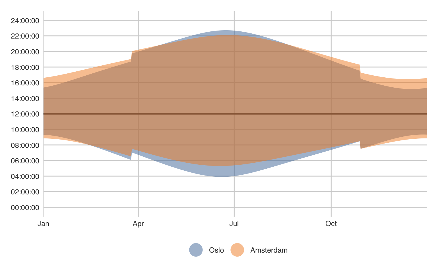
As you see, in neither cities 12:00 in the afternoon is perfectly in the middle between sunrise and sunset, although this trend is slightly enhanced for Oslo (again due to longitude differences). We can also see that the length of days in Oslo is longer in summer particularly because the mornings start earlier.

So let’s also squish everything on the bottom axis and just look at day length in total.

parse_sun_data(reticulate::py$df_deux) |>
  mutate(day_length = hms::as_hms(sunset - sunrise)) |>
  ggplot(aes(x = date, y = day_length, fill = city, group = city)) +
  geom_area(position = "identity", alpha = 0.5, key_glyph = "point") +
  labs(
    title = "Comparison in day length across the year",
    x = NULL,
    y = "Day length (_hours_)",
    fill = NULL
  ) +
  scale_x_date(labels = scales::label_date(format = "%B")) +
  scale_y_time(
    labels = scales::label_time(format = "%H hours"),
    limits = parse_time(c("00:00", "23:59"), "%H:%M"),
    breaks = hms::hms(hours = seq(0, 24, 4)),
    expand = expansion(add = 0)
  ) +
  ggthemes::scale_fill_tableau(guide = guide_legend(
    override.aes = list(shape = 21, size = 8), direction = "vertical"
  )) +
  theme_custom() +
  theme(
    plot.title.position = "plot",
    axis.title.y = element_markdown(),
    legend.position = c(0.85, 0.85)
  )

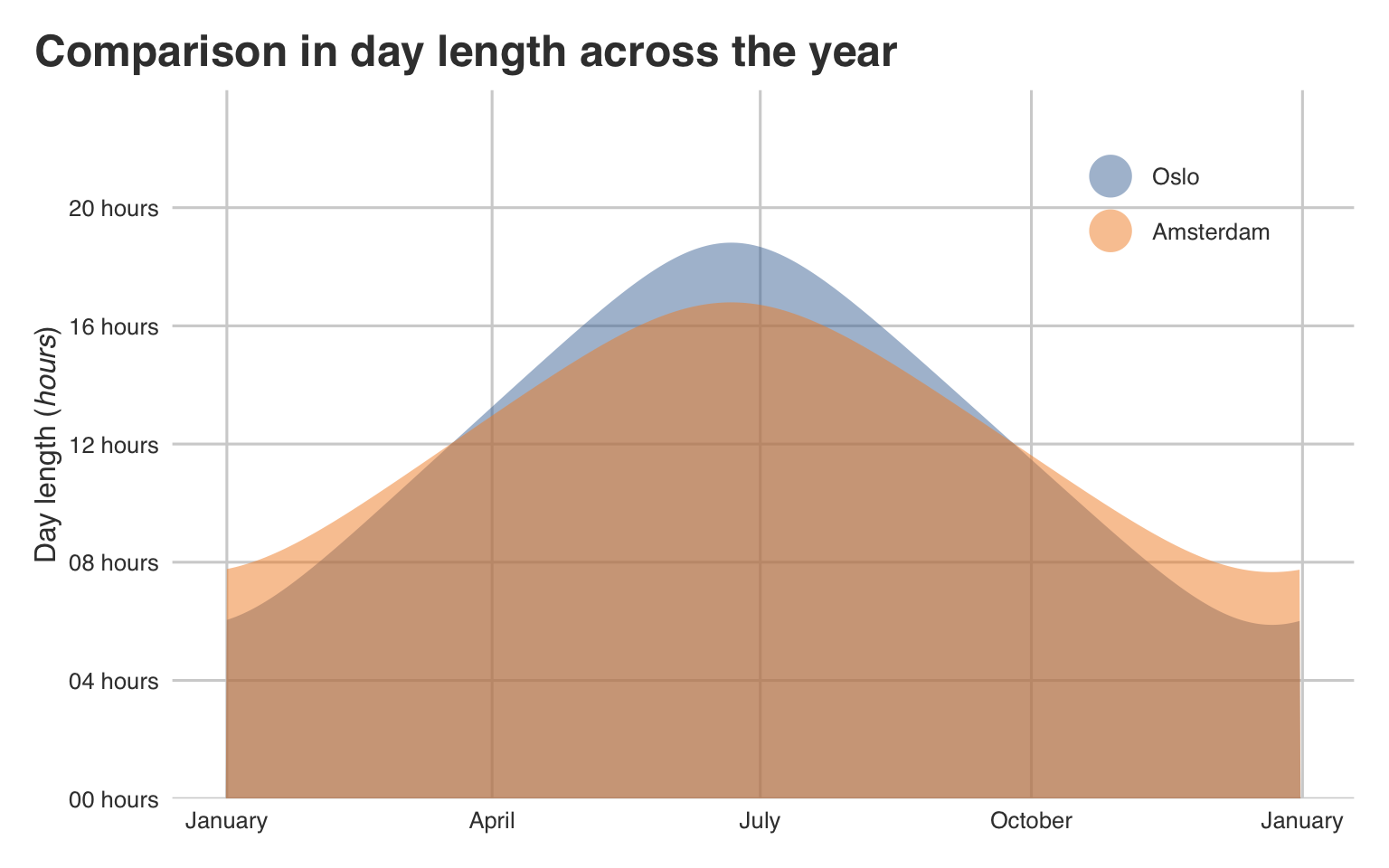
Now I’m curious when the largest difference occurs and when the days are roughly equal. Let’s select the relevant columns and get the day length in Oslo and Amsterdam next to each other using the pivot_wider() function so we can easily compare. Let’s then select the largest and smallest differences.

day_length_diff <- parse_sun_data(reticulate::py$df_deux) |>
  select(city, date, day_length) |>
  group_by(city) |>
  pivot_wider(
    id_cols = date, names_from = city, values_from = day_length,
    names_glue = "day_length_{city}"
  ) |>
  janitor::clean_names() |>
  mutate(difference = hms::as_hms(day_length_oslo - day_length_amsterdam))

print("Biggest positive difference:")
print(day_length_diff |> slice_max(difference))

print("Biggest negative difference:")
print(day_length_diff |> slice_min(difference))

print("Smallest differences:")
print(day_length_diff |> slice_min(abs(difference), n = 5))

[1] "Biggest positive difference:"
# A tibble: 1 × 4
  date       day_length_oslo day_length_amsterdam difference
  <date>     <time>          <time>               <time>    
1 2023-06-21 18:48:57        16:47:42             02:01:15  
[1] "Biggest negative difference:"
# A tibble: 1 × 4
  date       day_length_oslo day_length_amsterdam difference
  <date>     <time>          <time>               <time>    
1 2023-12-22 05:52:47        07:39:53             -01:47:06 
[1] "Smallest differences:"
# A tibble: 5 × 4
  date       day_length_oslo day_length_amsterdam difference
  <date>     <time>          <time>               <time>    
1 2023-03-19 12:04:45        12:04:28              00'17"   
2 2023-09-25 12:00:42        12:01:18             -00'36"   
3 2023-09-24 12:06:04        12:05:20              00'44"   
4 2023-03-18 11:59:17        12:00:22             -01'05"   
5 2023-03-20 12:10:12        12:08:35              01'37"   

Seems like the largest difference occur around the 20th of June when Oslo gets about 2 full hours of daylight more than Oslo.

Finally, let’s look at the effect of longitude (how far east or west a place is) on the sunset/sunrise times. The easiest way to look at this is to compare the time solar noon happens. Due to (most of) mainland Europe being in the same time zone (CET), it’s 12:00 at the same time across central Europe. However, the sun did not get the note and still travels (from Earth perspective) in a very consistent pace from east to west. This means that the sun arrives first in Poland and leaves last in Spain. This means that solar noon is unequal across the continent. Let’s look at when solar noon happens across the four cities in this analysis.

data |>
  ggplot(aes(x = date, y = noon, group = city, color = city)) +
  geom_hline(yintercept = hms::hms(hours = 12), linewidth = 1) +
  geom_line(linewidth = 2, key_glyph = "point") +
  labs(
    title = "What time is solar noon?",
    color = NULL
  ) +
  scale_x_date(expand = expansion(add = 0)) +
  scale_y_time(
    limits = hms::hms(hours = c(11, 15)),
    breaks = hms::hms(hours = seq(11, 15, 0.5))
  ) +
  ggthemes::scale_color_tableau(guide = guide_legend(
    override.aes = list(size = 4)
  )) +
  ggthemes::scale_fill_tableau() +
  theme_custom()

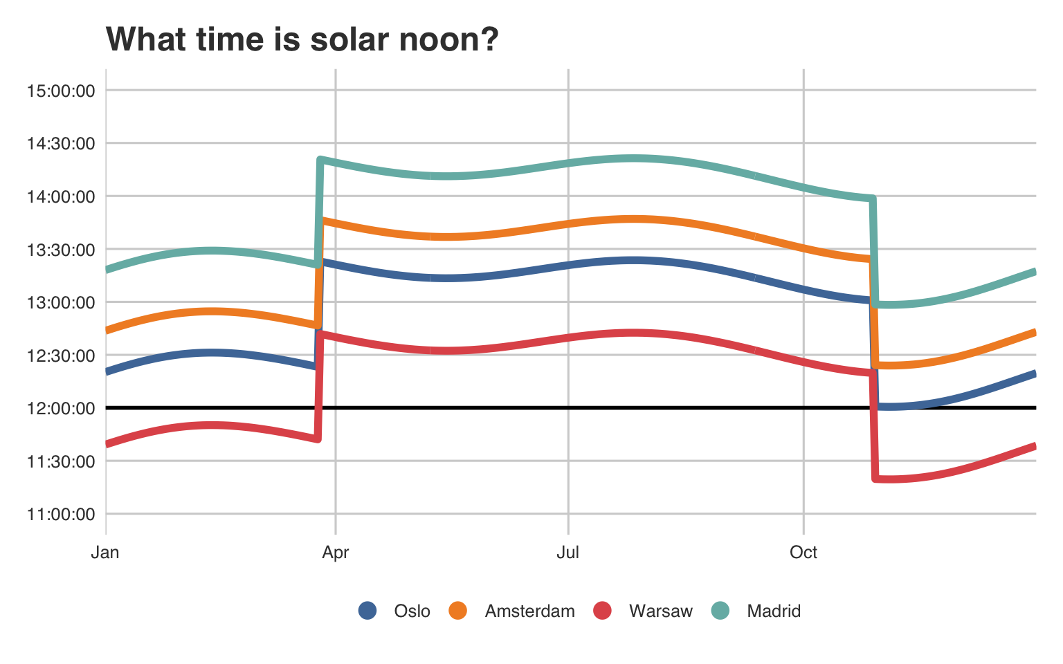
This one actually quite surprised me! Due to it’s location on the far west of the time zone Madrid has solar noon only at around 14:00. Oslo and Warsaw are actually the only cities that are at time roughly near the 12:00 mark corrected for DST. However, with DST Oslo has solar noon close to midday (12:00) in late October right after switching off from DST and Warsaw most of the winter months early in the year. Also, solar noon in Madrid is nearly 2 hours later than solar noon in Warsaw, which is quite a big difference for a single time zone, which is one of the few reasons Portugal is in the western European time zone)

If I had time (and motivation) I would explore some other extremes like China which one uses a single time zone despite probably needing 4 to 5 due to its size, Australia with it’s half hour time zones, and locations that are on roughly the same longitude but aren’t in the same time zone due to economic and/or political reasons (e.g. China, and Iceland which doesn’t observe DST). This was a fun little project, I certainly gained some insight into how latitude and longitude affect sunrise and sunset times and how much of a difference exists within central Europe. For an added bonus we got to create some fun plots, what’s not to love! Thanks for reading!