Introduction

Most people in my environment know R as the quintessential tool for statistical analysis and data visualization. There’s plenty of tutorials and discussions online about how to go about either. But one important aspect that is noticeably lacking is a discussion about R’s ability to simulate scenes from Star Wars. Today, we’ll set this straight. At the same time we’ll also explore how to incorporate a mathematical formula with a set of simple rules into R. This post is an R implementation of a formula published on the On-line Encyclopedia of Integer Sequences (OEIS, sequence A117966). Numberphile has a video from Brady Haran with Neil Sloane where they discuss the mathematics behind fun graphs, among which this one. It’s a great video, you can check it out here.

We’ll use a formula called the balanced ternary enumeration. The game is to convert a decimal number to base 3, or the ternary. The best way to describe the ternary is to put it next to the binary. Binary (or base 2) is perhaps more widely understood. I don’t actually know of any use of the ternary outside of these hypothetical mathematical problems. Octadecimal and hexadecimal are used sometimes. The latter is used for instance in defining colors in computers.

Let’s start with counting

Let’s start at the very basics. Like primary school basic. In the decimal system, we could from 1 to 9 and then add a digit and start from 1 again ([1 2 3 … 8 9 10 11 12 … 20 21 …]) This system likely comes from the fact that humans have 10 fingers. (Interestingly, the Maya used a system with base 20, because they used their toes to count also, and there’s a Native American tribe in California that uses base 8 because they use the space between fingers to count.) Computers use binary (base 2) because a pin or electrical signal can either be on or off. This means that there’s two values available to denote a number, either 0 or 1. In this system each digit represents the double of the previous, starting from 1. So the first digit represents 1, the second 2, the third 4, the fourth 8 and so on. So the number 5 is made from adding 4 and 1 together, so the binary representation of the number 4 is 100, and 5 is 101. The number 6 is denoted as 110, and so on. In a ternary system, this same principle applies as in the binary system, except digits now increase by a factor of 3. The first digit represents 1, the second 3, the third9 and so on. This also means that there’s three possible values to denote a number, 0, 1, or 2. To illustrate how decimal numbers are represented in the binary and ternary system, look at the table below.

Moving numbers between systems

Unlike MATLAB (dec2bin()) or Python (bin()), R doesn’t have a natural built-in function to convert decimal numbers to binary (unless you want to use the weird intToBits() function). So I wrote a function instead which continually appends the modulus while it loops through the digits of the numbers by dividing it in half continuously. The modulus is what is left after division of number x by number y. Let’s take the number 13 as an example. In the first loop, the modulus of 13 when divided by 2 is 1. So that goes in the first position, representing value 1. The next digit in the binary system represents the value 2. So we divide our initial value by 2 (and round it to the lower integer it in case we get decimal points) and take the modulus again. So the modulus of 6 when divided by 2 is 0. So that’s the second digit. The next loop will result in another 1 ($x = 6; \lfloor x/2 \rfloor\mod 2 = 1$), $\lfloor x \rfloor$ represents rounding $x$ to the nearest lower integer, i.e. floor), and then in the final loop, we take half of 3 and take the modulus again ($x = 3; \lfloor x/2 \rfloor\mod 2 = 1$). After this, when we floor 0.5, the loop cancels since from here on it will just produce an infinite amount of leading zero’s. This function now gives us the value 1101, which corresponds to the table above. The code for this function looks like this:

convert_to_binary <- function(x) {
  out <- mod <- NULL
  while (x > 0 || is.null(mod)) {
    mod <- x %% 2
    out <- paste0(mod, out)
    x <- floor(x / 2)
  }
  return(out)
}

Let’s run this function:

convert_to_binary(13)

[1] "1101"

Now in this function we’ve hard coded that the base is 2, but this code works for any base up to base 10 with just a simple rewrite of the code. If we go higher, e.g. base 11, we are going to have to start using letters to represent values, which I’m too lazy to implement right now. We can specify the base as an input variable.

convert_to_base_n <- function(x, base = NULL) {
  if (base > 10) {
    stop("Function not defined for bases higher than 10")
  }
  out <- mod <- NULL
  while (x > 0 || is.null(mod)) {
    mod <- x %% base
    out <- paste0(mod, out)
    x <- floor(x / base)
  }
  return(out)
}

These functions only accepts a single value, but to get the transformed value for a vector of integers we can use the map() function from {purrr}. map() as default outputs a list, but we can also ask for a character vector. We can then convert a number of values to binary like this:

example_vector <- c(seq(4), 10, 13, 22, 50, 75, 100)
map_chr(example_vector, convert_to_binary)

 [1] "1"       "10"      "11"      "100"     "1010"    "1101"    "10110"  
 [8] "110010"  "1001011" "1100100"

map_chr(example_vector, base = 3, convert_to_base_n)

 [1] "1"     "2"     "10"    "11"    "101"   "111"   "211"   "1212"  "2210" 
[10] "10201"

The rules of the game

Okay, so here’s the rules of the balanced ternary enumeration game We write all integers in base 3, and replace all digits that are 2 with -1 and then sum the outcome. Let’s look at the first ten numbers in ternary:

map_chr(seq(10), base = 3, convert_to_base_n)

 [1] "1"   "2"   "10"  "11"  "12"  "20"  "21"  "22"  "100" "101"

So in this sequence, we would replace the second value (2) with -1, which makes -1. We would also replace the second digit of fifth value (12), which makes [1,-1], which, when we add these numbers up , makes 2. This because 1 in the first position denotes value 3, minus 1 in the second position (representing 1) makes 2 since $(3 * 1) + (1 * -1) = 2$. The next value (20) has a 2 in the first position, replace this with -1 makes [-1,0]. The first position denotes 3, minus 0 in the second position, makes -3 since $(3 * -1) + (1 * 0) = -3$.

Applying the same rule to the sixth value gives $(3 * -1) + (1 * 1)$ which makes -2. The next value has two incidences of the number 2, replacing both with -1 gives $(3 * -1) + (1 * -1)$ is equal to -4. Let’s skip ahead a few numbers to decimal number 18, which in ternary becomes 200, where the first position represents the number 9. Replacing the 2 in this number gives $(9 * -1) + (3 * 0) + (1 * 0)$, which makes -9. This process is the balanced ternary enumeration.

Just as show of proof, we can also apply the same formula to values that don’t contain a 2, for instance decimal number 10, which becomes 101 in ternary. The formula for this becomes $(9 * 1) + (3 * 0) + (1 * 1)$, which makes again 10.

Let’s put this sequence together:

[0   1   -1   3   4   2   -3   -2   -4   9   10]

And that’s balanced ternary enumeration.

Coding the formula

So obviously we are lazy, and don’t want to do this process manually for thousands of values. that’s why we’re going to code it. For this step I translated some Python code to R syntax. The function I wrote to do one step of balanced ternary enumartion is shown below. The first value is always 0 (since it’s a 0 in the first position, hence $1 * 0 = 0$). After this, we can incorporate the two steps (of converting into ternary and the enumeration) into one. The formula for this looks like this:

$$ \begin{aligned} a(0) &= 0\newline a(3n) &= 3 * a(n)\newline a(3n + 1) &= 3 * a(n) + 1\newline a(3n + 2) &= 3 * a(n) - 1 \end{aligned} $$

In the function, since 0 will always result in 0, this is hard coded in. Afterwards it is a nested function (I know, we all love it) where it iteratively calls itself until the input to the function is 0 and it stops. At that point we have out balanced ternary. This function only performs the calculation for one value. So getting a sequence means putting it in a map() function.

bte <- function(x) {
  if (x == 0) {
    return(0)
  }
  if (x %% 3 == 0) {
    return(3 * bte(x / 3))
  } else if (x %% 3 == 1) {
    return(3 * bte((x - 1) / 3) + 1)
  } else if (x %% 3 == 2) {
    return(3 * bte((x - 2) / 3) - 1)
  }
}

def bte(x):
  if x == 0: 
    return 0
  if x % 3 == 0:
    return 3 * bte(x / 3)
  elif x % 3 == 1:
    return 3 * bte((x - 1) / 3) + 1
  else:
    return 3 * bte((x - 2) / 3) - 1

Let’s go through one iteration of this code. Let’s say x <- 3. 3 modulo 3 is equal to 0, so we enter the first condition. The result of this is 3 multiplied by the outcome of the same function, except the input now is x divided by three, or 3/3, or 1, in our example. This becomes the new input for the function. 1 modulo 3 is equal to 1. So now we enter the second condition. Now the input to the bte() function is 1 minus 1, divided by 3. This is 0, so we return 3 * 0 + 1, which is equal to 3.

If we plug the number 3 into the formula, we will get the same result:

bte(3)

[1] 3

Let’s also look at a few other examples using the map() function again. Since the bte() function outputs only integers, I use map_dbl(). Let’s input a few examples:

example_vector <- c(0, seq(10), 500, 1500, 9999)
map_dbl(example_vector, bte)

 [1]    0    1   -1    3    4    2   -3   -2   -4    9   10 -232 -696 9270

This corresponds to the values we created earlier, and the larger numbers make sense also. Okay, let’s now create an entire sequence. We’ll do 59.048 iterations (it’ll become clear later why this specific number). We’ll save the output in a variable called starwars_seq (forgotten yet that this thing started with Star Wars?).

starwars_seq <- map_dbl(seq(59048), bte)

Plotting the Star Destroyers

Now, when we plot the values as a scatter plot, it’ll become maybe a bit clearer how this mathematical formula circles back to our Star Wars scene.

ggplot(data = NULL, aes(x = seq(starwars_seq), y = starwars_seq)) +
  geom_point() +
  theme_minimal()

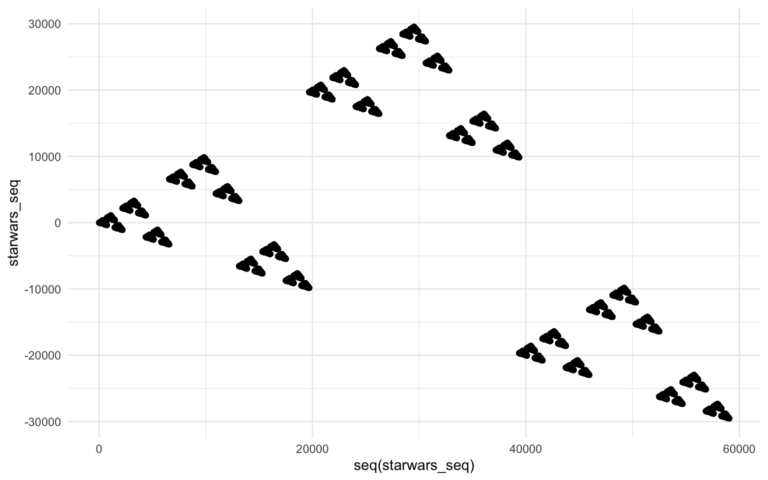
It’s star destroyers in battle formation! How crazy is that!? It’s such an interesting pattern. You can create as many formations as you like (or as your computer can handle) since the sequence will continue to infinity (it’s like Emperor Palpatine’s wet dream). Another feature of this sequence is that it will return every integer exactly once. We can confirm this property very easily by comparing the number of integers given to the balanced ternary enumeration function and the length of unique values returned:

length(starwars_seq) == length(unique(starwars_seq))

[1] TRUE

The first point of each “squadron” of star destroyers starts with a value that is the same in decimal system as it is in balanced ternary enumeration. Remember the length of the starwars_seq variable was 59 048? I chose that because it would start plotting a new squadron at x = 59049. Let’s confirm this:

bte(59049)

[1] 59049

There is a range of values where the input of the balanced ternary enumeration is equal to the outcome (or where the outcome is equal to the input divided by two times -1 ($\frac{-x}{2}$). There’s a clear pattern to these numbers, but I’ve done enough maths for today, so I’ll save it for another time.

Anyway, the plot! It is cool and all, but let’s make it look a bit more like Star Wars by changing some style elements. We’ll also generate some stars. For fun’s sake we’ll also add a planet or moon.

set.seed(1983)

ggplot(data = NULL, aes(x = seq(starwars_seq), y = starwars_seq)) +
  geom_point(
    aes(
      x = sample(seq(-1e4, length(starwars_seq) + 1e4), 1e3),
      y = sample(seq(
        min(starwars_seq) - 1e4,
        max(starwars_seq) + 1e4
      ), 1e3),
      size = sample(runif(length(starwars_seq) + 1e4), 1e3)
    ),
    shape = 18, color = "yellow"
  ) +
  geom_point(
    aes(
      x = sample(seq(starwars_seq), 1),
      y = sample(starwars_seq, 1)
    ),
    shape = 19, size = 12, color = "darkslategray"
  ) +
  geom_point(size = 4, color = "grey90") +
  scale_size_continuous(range = c(1e-3, 5e-1)) +
  theme_void() +
  theme(
    legend.position = "none",
    panel.background = element_rect(fill = "black")
  )

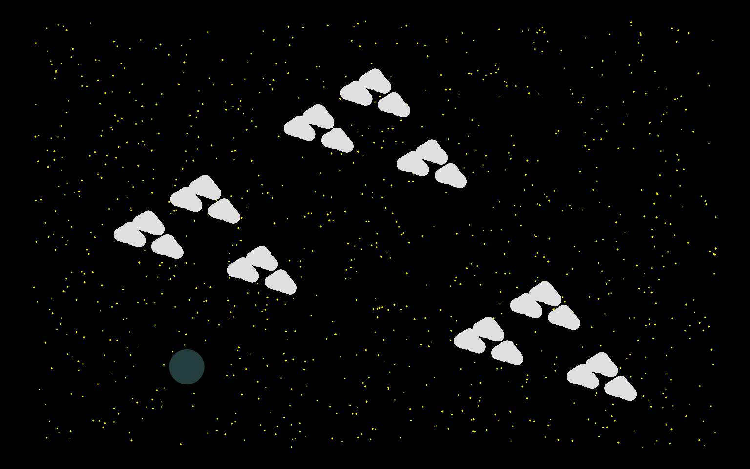
Hope you enjoyed reading about me rambling about maths and implementing these functions to R! I will certainly do another plot some time later!

BONUS
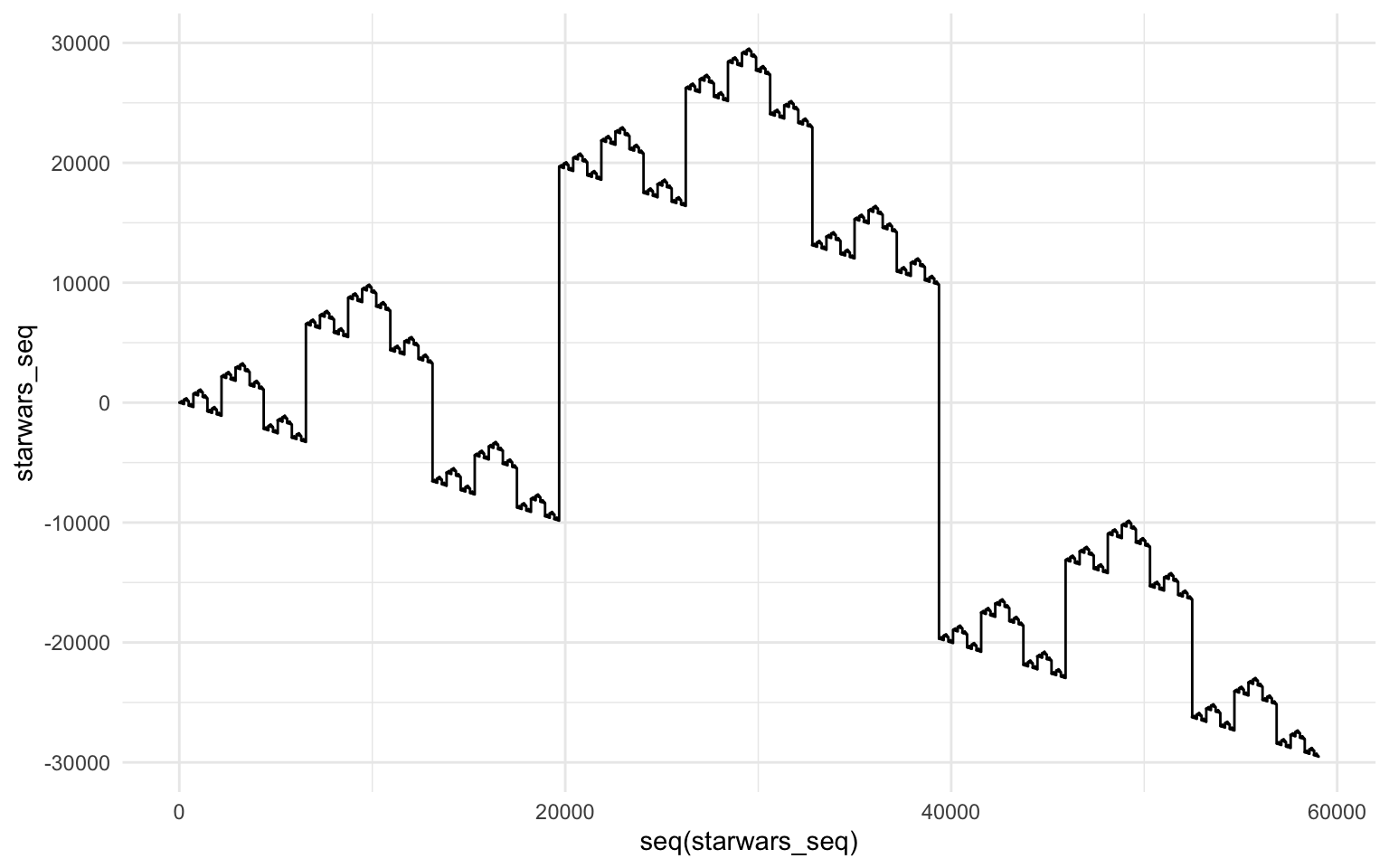
We can create another plot (nothing related to Star Wars perhaps), that looks nice also. Now, instead of geom_point() we’ll use geom_line(). No further purpose, just pretty.

ggplot(data = NULL, aes(x = seq(starwars_seq), y = starwars_seq)) +
  geom_line() +
  theme_minimal()